https://venturaphotonics.com/research-page-6.html
REJECT AR6
Ventura Photonics Climate Post 006.1a Feb. 20 2022
By Dr. Roy Clark – Dr. Roy Clark, founder and president of Ventura Photonics has over 30 years of experience in optics and spectroscopy with emphasis on new product and process development for adverse environments. He has 8 US Patents in the areas of illumination, higher energy lasers, optical sensors and optics components.

The Sixth IPCC Climate Assessment Report (AR6) should be rejected outright because it is based on the use of fraudulent climate models. This fraud comes from the underlying assumption of radiative forcing in an equilibrium climate used to construct the models. Such models are fraudulent by definition, before a single line of computer code is written. Climate science has now degenerated past scientific dogma into the quasi-religious ‘Imperial Cult of the Global Warming Apocalypse’. Scientific reason has been replaced by blind advocacy. There is no ‘climate crisis’. Eisenhower’s warning about the corruption of science by government funding has come true. The entire multi-trillion dollar Ponzi or pyramid scheme built on these fraudulent modeling results needs to be shut down and those responsible should face the legal consequences of their activities.
SUMMARY
The recently published draft of the latest UN Intergovernmental Panel on Climate Change (IPCC) Report, Climate Change 2021: The Physical Science Basis, [IPCC, 2021] the contribution of Working Group 1 to the Sixth IPCC Climate Assessment (AR6) should be rejected outright because the report is based on the results from fraudulent climate models. This fraud comes from the underlying assumption of radiative forcing in an equilibrium average climate used to construct the climate models. These models are fraudulent by definition before any computer code is even written. AR6 is a continuation of the climate modeling fraud that started with the invalid assumptions that were made when the first computer climate models were developed in the 1960s. All of the equilibrium climate model results used by the IPCC since it was established in 1988 are fraudulent.
There are at least three separate parts to this fraud. First there are the invalid climate equilibrium and related assumptions that originated in the nineteenth century. These led to melodramatic prophecies of the global warming apocalypse and became such a good source of research funding that the scientific process of hypothesis and discovery collapsed. Second, there was institutional fraud related to ‘mission creep’ within various government agencies. For example, NASA was established to put a man on the moon. There was no provision to shut it down after that mission was accomplished. Climate modeling provided alternative employment for some of the NASA ‘scientists’ with nothing else to do. The climate fraud was firmly established at NASA by 1981. Third, there was a deliberate decision by various outside interests, including environmentalists and politicians to exploit the climate apocalypse to further their own causes. There was no single person or event that created the climate fraud. There was a gradual transition from the invalid hypothesis of an equilibrium average climate to the massive multi-trillion dollar pyramid or Ponzi scheme that we have today.
The peer review process in climate science has collapsed and been replaced by blatant cronyism. The climate modelers have retreated inside a cocoon of lies where they discuss the pseudoscience of radiative forcings, feedbacks and climate sensitivities to a CO2 ‘doubling’. This is just climate theology. How does a doubling of the atmospheric CO2 concentration change the number of angels that may dance on the head of a climate pin? Here they use their ‘advanced’ climate models to create the sacred spaghetti plots of global warming. This is GIGO: garbage in, gospel out. The model ‘predictions’ are fed directly to government agencies and the IPCC with minimal outside scrutiny. There is no climate science involved. Irrational belief in computer models has replaced the Laws of Physics. The Imperial Cult of the Global Warming Apocalypse has claimed the Divine Right to save the world from a non-existent problem. There is no ‘climate crisis’. Eisenhower’s warning about the corruption of science by government funding has come true. The entire multi-trillion dollar Ponzi or pyramid scheme built on these fraudulent modeling results needs to be shut down and those responsible should face the legal consequences of their activities.
TECHNICAL SUMMARY
The fundamental scientific error in the climate models is the climate equilibrium assumption. This has been used to oversimplify the energy transfer processes that determine the surface temperature. It creates the illusion that the surface temperature is determined by the LWIR flux. In reality, a change in surface temperature has to be determined from the change in enthalpy or heat content of the surface thermal reservoir divided by the heat capacity. Any small change in LWIR flux from a so called ‘radiative forcing’ has to be added to the rest of the flux terms in an interactive, time dependent thermal engineering calculation of the surface temperature. There are four main flux terms, the solar heating, the net LWIR emission, the moist convection (evapotranspiration) and the subsurface thermal transport. Furthermore, the LWIR flux cannot be separated and analyzed independently of the other flux terms. It is fully coupled to the moist convection.
There is an abundance of evidence that clearly demonstrates that the equilibrium climate assumption is invalid. However, this has been ignored by the climate modeling community. Fourier described time delays or phase sifts between the peak solar flux and the subsurface seasonal temperature response in 1824. Such phase shifts can be found in the seasonal and daily temperature changes in both land and ocean temperatures. They are definitive evidence of non-equilibrium thermal response. These phase shifts alone are sufficient to invalidate the equilibrium climate models. In addition, there are also quasi-periodic ocean oscillations that provide a ‘noise floor’ for climate temperature variations.
The idea that changes in the atmospheric concentration of CO2 could cause the earth to cycle through an Ice Age was first proposed by Tyndall in the 1860s. This was finally disproved in 1976 when the 100,000 year Ice Age cycle was linked to changes in the earth’s orbital eccentricity through the analysis of deep drilled ocean sediment cores. If changes in atmospheric CO2 concentration do not cycle the earth through an Ice Age then there is no reason to expect that changes in CO2 concentration from fossil fuel combustion should have any effect on climate.
Simple energy balance calculations show that the long term planetary average LWIR flux returned to space should be near 240 W m-2. Satellite radiometer measurements give a value of 240±100 W m-2. However, this is simply a cooling flux that does not define an emission temperature. The spectral distribution is not that of a blackbody near 255 K. This means that there can be no ‘equilibrium greenhouse effect temperature’ of 33 K. All of the ‘discussion’ over a ‘greenhouse effect temperature’ is nothing more than climate theology.
The underlying assumption used in equilibrium climate modeling is that there exists an ‘equilibrium average climate’ with an exact flux balance at the top of the atmosphere (TOA) between the absorbed solar flux and the LWIR flux emitted to space. An increase in atmospheric CO2 concentration reduces the LWIR flux within the CO2 emission bands. This is called a ‘radiative forcing’. It is then assumed that this is a perturbation to the climate equilibrium state. The surface temperature is then supposed to ‘adjust’ to a new higher temperature to restore the flux balance at TOA. It is also assumed that the surface temperature response is linear and that there is an amplification of the warming by a ‘water vapor feedback’. A doubling of the CO2 concentration from a ‘preindustrial level’ of 280 parts per million (ppm) to 560 ppm produces a ‘radiative forcing’ of 3.7 W m-2. A pseudoscientific ‘climate sensitivity’ to CO2 is then used to create an increase in ‘equilibrium surface temperature’ of 3.7 ±1.9 C.
In reality, a change in flux produces a change in the rate of heating or cooling, not a change in temperature. The ‘radiative forcing’ at TOA is produced by absorption at lower levels in the atmosphere mainly by the P and R braches of the main CO2 band near 640 and 700 cm-1. The maximum increase in the rate of heating for a ‘CO2 doubling’ is near 0.08 K per day at an altitude near 2 km. This is coupled to the normal convective motion in the troposphere. At an average lapse rate of 6.5 K km-1 this corresponds to a decrease in altitude of about 12 meters. This is equivalent to riding an elevator down about 4 floors. The small amount of heat produced at each level in the troposphere is dissipated by a combination of broadband emission, mainly by the water bands and a slight increase in the gravitational potential energy. It does not couple to the surface. There is no change to the ‘energy balance’ of the earth, the absorbed LWR flux is just rearranged and emitted at different wavelengths.
Although it is not explicitly discussed by the IPCC as part of radiative forcing, there is also an increase in the downward LWIR flux to the surface that is similar in magnitude to the reduction in LWIR flux at TOA. The radiation field in the atmosphere consists of many thousands of overlapping lines. Each line corresponds to a transition between two vibration-rotation states of a so called ‘greenhouse gas’. The dominant greenhouse gas molecules are water vapor and CO2. In the lower troposphere the lines are pressure broadened. Within the main absorption-emission bands, the lines merge to form a quasi-continuous blackbody source. Because of these line broadening effects, almost all of the downward LIWR flux to the surface originates from within the first 2 km layer above the surface and approximately half of the LWIR flux originates from within the first 100 m layer. This means that the LWIR emission to space is decoupled from the downward LWIR flux to the surface.
The troposphere functions as an open cycle heat engine that divides naturally into two independent thermal reservoirs. The lower reservoir extends from the surface to an altitude near 2 km. The upper thermal reservoir extends from 2 km to the tropopause. The upper reservoir is the cold reservoir of the heat engine. As the warm moist air rises from the surface by convection, the air expands and cools. The some of the internal molecular heat energy is converted to gravitational potential energy. As the air cools by LWIR emission at higher altitudes in the troposphere, it sinks and gravitational potential energy is converted back to heat. If the air is moist, water vapor condenses above the saturation level. Clouds form and latent heat is released. For dry air, the lapse rate or temperature profile for convective ascent is -9.8 K km-1. For moist air the magnitude of the lapse is reduced because of the latent heat release. The US standard atmosphere uses an average moist lapse rate of -6.5 K km-1. In addition, air can be compressed and heated by a downward flow. This occurs in high pressure systems and with downslope winds. Near surface air temperatures may change by 10 C over a short time period from hours to a few days.
The greenhouse effect is simply the LWIR exchange energy at the surface. The downward LWIR flux from the lower troposphere ‘blocks’ most of the upward LWIR flux the surface. There is an exchange of photons but much reduced heat transfer. In order to dissipate the absorbed solar flux, the surface must warm up so that the excess heat is dissipated by moist convection. In addition, some of the heat may be transported and stored below the surface. The land and ocean surfaces have different thermal properties and have to be analyzed separately.
Over land, almost all of the absorbed solar heat is dissipated within the same diurnal cycle. As the surface warms during the day, the excess heat is removed by moist convection. Some of the heat is conducted below the surface, stored and returned to the surface later in the day. In the evening, the surface cools and the convection essentially stops as the surface and air temperatures equalize. The surface then cools more slowly over night by net LWIR emission. The equalization or convection transition temperature is reset each day by the local weather system passing through. The day to day changes in the convection transition temperature are sufficiently large that any change in surface temperature from an in increase in the downward LWIR flux from CO2 is too small to measure. There can be no CO2 induced temperature ‘signal’ in the weather station data used to create the average surface temperature anomaly.
Over the oceans, the water surface is almost transparent to the solar flux. Approximately 90% of the solar flux is absorbed within the first 10 m layer of the ocean. The diurnal temperature rise is small and the bulk ocean temperature increases until the excess solar heat is dissipated by wind driven evaporation. The cooler surface water sinks and is replaced by warmer water from below. This allows the evaporation to continue at night. Within the ±30° latitude bands the sensitivity of the evaporation to the wind speed is approximately 15 W m-2/m s-1. The latent heat flux increases by 15 W m-2 for an increase in wind speed of 1 m s-1. The penetration depth of the LWIR flux into the ocean surface is 100 micron or less. Here the LWIR flux is fully coupled to the wind driven cooling flux. The two should not be separated and analyzed separately. There can be no measurable ocean warming from CO2. The magnitude and variability in the wind driven latent heat flux are too large. The average increase in atmospheric CO2 concentration is approximately 2.4 ppm per year. This produces an increase in downward LWIR flux to the surface of 0.034 W m-2. This is equivalent to a change in wind speed of 2.3 mm per year.
1.0 INTRODUCTION
Over the last 200 years, the atmospheric concentration of CO2 has increased by approximately 130 ppm from 280 to 410 ppm as shown in Figure 1a [Keeling, 2021]. This has been attributed to increases in fossil fuel combustion since the start of the industrial revolution [Meinshausen et al, 2011]. Countries such as China and India are still building new coal fired electrical power generation plants, so the atmospheric CO2 concentration will continue to increase [BP, 2020]. The LWIR flux in the atmosphere can be calculated using high resolution radiative transfer algorithms and HITRAN or a similar spectroscopic database [HITRAN, 2020, Wijngaarden and Happer, 2020]. The results of such calculations from Harde [2017], Hansen [2005] and Clark [2013] are shown in Figure 1b. This shows the change in total LWIR flux. Most of this occurs within the P and R branches of the v2 CO2 band near 640 and 700 cm-1. There is also a small contribution from the overtone bands near 950 and 1050 cm-1. There is good agreement between the different calculations. As the CO2 concentration increases, there is a slight increase in the downward LWIR flux reaching the surface and a small decrease in the LWIR flux emitted at TOA. For the observed increase of 130 ppm, the change in flux is approximately 2 W m-2. For a doubling of the CO2 concentration from ‘preindustrial’ levels of 280 ppm to 560 ppm, the decrease at TOA is given as 3.7 W m-2 [IPCC 2013] or 3.9 W m-2 [IPCC, 2021] and for a doubling from 360 to 720 ppm, the decrease is near 5 W m-2. The calculated change in LWIR flux may vary slightly depending on the surface temperature and humidity values selected. Currently, the average increase in atmospheric CO2 concentration is near 2.4 ppm per year and the increase in downward flux to the surface is approximately 0.034 W m-2 per year.


Figure 1: a) The increase in atmospheric CO2 concentration from 1800 and b) calculated changes in atmospheric LWIR flux produced by an increase in atmospheric CO2 concentration from 35 to 760 ppm.
The issue therefore is not the value of the change in atmospheric LWIR flux produced by an increase in atmospheric CO2 concentration, but the effect of this change on the earth’s climate, starting with the calculation of the increase in surface temperature. Here there is complete disagreement between the conventional thermal engineering approach and the equilibrium radiative forcing techniques used in the climate models [Poyet, 2020, Gerlich and Tscheuschner, 2009].
In the real world, the surface temperature is determined by the interaction of four main time dependent heat flux terms with the surface thermal reservoir. These are the absorbed solar flux, the net LWIR emission, the evapotranspiration (moist convection) and the subsurface thermal transport. (Rainfall and freeze/thaw effects are not included here). A change in temperature is determined by dividing the change in heat content or enthalpy by the local heat capacity of the thermal reservoir. In order to determine the effect of an increase in atmospheric CO2 concentration on the surface temperature, the change in enthalpy has to be determined after a solar thermal cycle with increased downward LWIR flux from CO2. There are two parts to this analysis. First, the change in temperature from the small increase in downward LWIR flux from CO2 has to be evaluated. Second, the effect of other processes such as changes in local weather conditions have to be evaluated to determine if the CO2 induced changes are even measurable. In signal processing terms, this is the determination of the signal to noise ratio. The results of such calculations show that the increase in surface temperature produced by the increase in downward LWIR flux from CO2 is too small to measure.
The climate models start from the invalid concept of an equilibrium average climate. It is assumed that there is an exact long term planetary energy balance between the average absorbed solar flux and the average outgoing LWIR radiation (OLR) returned to space. An increase in the atmospheric CO2 concentration produces a slight reduction the LWIR flux at TOA within the CO2 emission band. This is considered to be a perturbation to the equilibrium state. The re-emission of the absorbed LWIR flux at other wavelengths and the coupling to the convection are ignored. The climate is then presumed to ‘adjust’ so that there is an increase in ‘equilibrium surface temperature’ that restores the flux balance at TOA [Knutti, and Hegerl, 2008]. The change in flux at TOA is called a radiative forcing. It is further assumed that there is a linear relationship between the ‘radiative forcing’ and the surface temperature response.

[Harde, 2017, IPCC, 2013 Chap. 8]. Climate sensitivity is defined in terms of the temperature change produced by doubling of the CO2 concentration from a ‘preindustrial’ level of 280 ppm to 560 ppm. It is assumed a-priori that all of the recent changes in temperature record must be attributable to the increase in ‘radiative forcing’. Effects such as natural oscillations in ocean surface temperatures are ignored.
2.0 ENERGY TRANSFER IN A NON-EQUILIBRIUM CLIMATE SYSTEM
In order to understand how the earth’s climate really works it necessary to introduce four concepts that are not part of a ‘climate equilibrium state’.
1) The so called ‘greenhouse effect’ has to be defined as the time dependent surface LWIR exchange energy.
2) There are significant phase shifts or time delays in the climate system between the peak solar flux and the surface temperature response.
3) The penetration depth of the LWIR flux into the oceans is approximately 100 micron. Here it is fully coupled to the wind driven evaporation or latent heat flux.
4) The land surface temperature is reset each day by the convection transition temperature.
These concepts will now considered in more detail.
2.1 The Greenhouse Effect
The earth’s surface is warmer than it should be based on rather simple energy conservation arguments. The average solar flux at the top of the atmosphere (TOA) is near 1368 W m-2. The exact value depends on satellite radiometer calibration [Wilson, 2014]. The albedo or reflectivity is near 0.3. The geometry is that of a sphere illuminated by a circular beam of nearly collimated solar radiation. The sphere to disk surface area ratio is four. This means that the average LWIR flux returned to space should be near 1368*(1-0.3)/4 ≈ 240 W m-2. IPCC AR6 gives 239 (237 to 242) W m-2. If the earth were a uniform blackbody emitter, this would correspond to an emission temperature near 255 K. Simple inspection of IR satellite images of the earth, such as the CERES image shown in Figure 2 indicates that the LWIR flux is approximately 240 ±100 W m-2 [CERES, 2011]. The various heating and cooling rates within the climate system interact to keep the surface temperature within the relatively narrow range needed to sustain the development of life on earth. These rates are always changing on diurnal, seasonal and longer time scales. There is no equilibrium.

Figure 2: CERES IR image of the earth, March 8, 2011
Furthermore, the spectral distribution of the LWIR flux emitted by the earth at the top of the atmosphere is not that of a blackbody. There is no ‘shell’ of gas surrounding the earth with a temperature near 255 K. The outgoing LWIR radiation (OLR) at TOA is simply the cumulative emission from many different layers of the atmosphere. The emission from each layer is modified by the absorption and emission of the layers above. These temperatures are also changing because of convective (vertical) motion in the troposphere. The spectral distribution of the OLR under ‘clear sky’ conditions is illustrated in Figure 3. The LWIR flux consists of a mix of atmospheric emission, mainly from the H2O and CO2 bands and surface emission through the LWIR transmission window. Some of the surface emission is absorbed by stratospheric ozone. The main spectral features are labelled. Blackbody emission curves at selected temperatures are also shown. The 255 K blackbody emission curve is shown as the black dotted line. It has no relationship to the TOA flux shown by the orange line. The LWIR flux at TOA is just a cooling flux that should not be used to define an ‘effective emission temperature’. This means that there can be no greenhouse effect temperature near 33 K [Taylor, 2006].

Figure 3: The LWIR flux emitted at TOA (orange line). The blackbody emission curves at selected temperatures are also shown. This TOA flux cannot be described as LWIR blackbody emission near 255 K. MODTRAN calculation, 288 K surface temperature, 80% RH, 400 ppm CO2, 100 to 1500 cm-1 spectral range, 2 cm-1 spectral resolution, mid latitude summer [MODTRAN, 2020].
It is also well known that the OLR at ‘clear sky’ increases linearly with surface temperature as shown in Figure 4 [Koll and Cronin, 2018]. There are two contributions to the OLR flux with different responses to the surface temperature. Within the LWIR transmission window in the 800 to 1200 cm-1 region, the surface emission is only partially absorbed and some is emitted to space. Here, the clear sky OLR increases linearly with surface temperature. Within the main H2O and CO2 absorption bands, the OLR emission does not change significantly with surface temperature. The water band emission profile shifts to higher altitude as the surface temperature increases. More heat is stored as gravitational potential energy. The LWIR absorption and emission process continues with increasing altitude until the molecular linewidths narrow sufficiently to allow the transition to a free photon flux to space. For H2O, this transition occurs near a temperature of 253 K (-20 C). For CO2 the free photon transition occurs at a lower temperature near 220 K (-53 C). Most of the CO2 band emission occurs in the stratosphere. This is shown below in Figure 12.

Figure 4: The increase in clear sky OLR flux with surface temperature
The observed linear increase in OLR flux in response to an increase in surface temperature does not mean that a change in OLR flux can couple back to the surface and change the surface temperature. This is a violation of the Second Law of Thermodynamics. Instead, the greenhouse effect is simply the result of the LWIR exchange energy at the surface. The downward LWIR flux from the lower troposphere ‘balances’ most the upward LWIR flux from the surface. Photons are exchanged without a net transfer of heat. When the surface and air temperatures are similar, the net LWIR flux limited to the LWIR transmission window, mainly in the 800 to 1200 cm-1 spectral region. The net LWIR flux increases with decreasing humidity and decreases with increasing cloud cover. This is illustrated in Figure 5. In order to dissipate the excess absorbed solar insolation, the surface warms up until the heat is removed by moist convection (evapotranspiration). This is a non-equilibrium process in which some of the absorbed solar heat is stored in the surface thermal reservoir and then released as the rates of heating and cooling change during the diurnal and seasonal cycles. In addition, some of the solar heat is stored below the ocean surface and can be transported over long distances by ocean currents. The energy transfer processes at the land-air and ocean–air are different, so the two have to be analyzed separately.


Figure 5: a) The surface exchange energy and b) MODTRAN calculation, using the same conditions as Figure 3.
The troposphere functions as an open cycle heat engine that transports part of the absorbed solar heat from the surface to the middle and upper troposphere by moist convection. From here it is radiated to back space, mainly by the water bands. Some of the surface heat is stored as gravitational potential energy in the troposphere. Convection is a mass transport process that is coupled to both the gravitational potential and the angular momentum or rotation of the earth. These interactions result in the formation of the Hadley, Ferrell and polar cell convective structure, the trade winds and the ocean gyre circulation. The ‘greenhouse effect’ is an integral part of the energy transfer processes that determine the earth’s weather patterns. The LWIR flux in the troposphere is part of the tropospheric heat engine and should not be separated and analyzed independently from the mass transport. The greenhouse effect is produced by the time dependent surface LWIR exchange energy on a rotating water planet.
2.2 The Time Delay or Phase Shift between the Peak Solar Flux and the Temperature Response
In order to warm or cool the surface thermal reservoir, heat must flow into or out of the reservoir. This introduces a time delay or phase shift between the peak solar flux and the temperature response. This type of phase shift also occurs on different time and energy scales in other energy storage devices. These include capacitors and inductors in electronic AC circuits and photon storage in passive optical resonators (cavity ringdown). This is not new science. The seasonal subsurface phase shift was described by Fourier in 1824 and 1827 [Fourier, 1824, 1827]. The most obvious phase shift is the seasonal delay between the peak solar insolation at summer solstice and the peak summer temperatures. At mid latitudes, this is usually between 4 and 8 weeks. Such phase shifts have been recorded by the weather stations for well over 100 years. Figure 6 shows the phase shifts for selected weather stations in S. California. These are the 30 year daily average MSAT Tmin and Tmax 1981-2010 climate data for Los Angeles, LA Airport (LAX), Redlands, Riverside, San Bernardino, Blythe, Indio and Mecca [WRCC, 2020]. The values of the phase shifts in days after summer solstice are shown in Figure 7. The observation of such phase shifts provides clear evidence of non-equilibrium thermal storage. This is sufficient to show that there is no equilibrium climate state that can be perturbed by an increase in the atmospheric CO2 concentration.


Figure 6: 30 year daily average MSAT Tmin and Tmax 1981-2010 climate data for selected weather stations in S. California. The seasonal phase shifts past summer solstice are clearly visible.

Figure 7: Seasonal phase shifts (days after summer solstice) for the weather station climate data shown in Figure 6.
Such phase shifts are also found in ocean temperature data. In fact the seasonal phase shifts are first generated by ocean solar heating. They are coupled to the weather station measurements through the diurnal convective transition temperature as the weather systems move over land. Figure 8 shows the monthly 2.5 m to 200 m depth ocean temperature profiles for 2018 for the N. Atlantic Ocean at 30° N, 20° W derived from Argo float data [Argo 2020]. The data are for a 5° x 1° (latitude x longitude) strip. The minimum winter surface temperature of 19 C is reached in March. Solar heating then produces a stable stratified thermal layer structure with a surface temperature peak of 24 C in August. The subsurface thermal layer structure then collapses as the wind driven evaporative cooling in winter exceeds the solar heating. The time delay or phase shift between the peak solar flux and the peak surface temperature response is approximately 8 weeks. These phase shifts increase with depth. At 60 m the phase shift is 16 weeks.

Figure 8: The 2.5 m to 200 m depth ocean temperature profiles for 2018 for the N. Atlantic Ocean at 30° N, 20° W derived from Argo float data [Argo 2020]. The data are for a 5° x 1° (latitude x longitude) strip. The seasonal phase shifts are indicated.
In addition to the seasonal phase shifts, there are also diurnal phase shifts in both the land and ocean temperatures that may reach 2 hours or more. However, such phase shifts were not usually recorded as part of the historical weather station record.
2.3 The Coupling of the LWIR Flux to the Oceans
The penetration depth of the LWIR flux into the ocean surface is approximately 100 micron (0.004 in). This is illustrated in Figure 9 [Hale and Querry, 1973]. Here it is fully coupled to the wind driven surface evaporation or latent heat flux. The sensitivity of the ocean latent heat flux to the wind speed may be estimated from the long term zonal data provided by Yu et al [2008]. This is shown in Figure 10. Over the ±30° latitude bands, the sensitivity is at least 15 W m-2/m s-1. As shown above in Figure 1b, the increase in downward LWIR flux to the surface produced by the observed 120 ppm increase in atmospheric CO2 concentration is approximately 2 W m-2. Within the ±30° latitude bands, this is dissipated by an increase in wind speed near 13 cm s-1. The average increase in CO2 concentration at present is near 2.4 ppm. This corresponds to an annual increase of 0.034 W m-2 in the downward LWIR flux to the surface. This is dissipated by an increase in wind speed near 2 millimeters per second.

Figure 9: Penetration depth of LWIR radiation into the oceans, a) 3300 to 50 cm-1 and b) 1200 to 200 cm-1. The locations of the main CO2 band and the overtones are indicated.

Figure 10: The sensitivity of the ocean latent heat flux to the wind speed.
…
7.0 CONCLUSIONS
The Sixth IPCC Climate Assessment (AR6) should be rejected outright because the report is based on the results from fraudulent climate models. The fundamental error is the underlying assumption of radiative forcing in an equilibrium average climate. There are no forcings, feedbacks or climate sensitivity to CO2 in the earth’s climate. The modern modeling fraud can be traced back to two papers, Manabe and Wetherald [1967] and Hansen et al [1981]. Between them, these papers contain seven fundamental scientific errors that provided the foundation for the multi-trillion dollar climate fraud we have today. The fraud has at least three different parts. First there is the technical fraud. This started in the nineteenth century with the equilibrium climate hypothesis and speculation that changes in the atmospheric concentration of CO2 could cause the earth to cycle through an Ice Age. Later, exaggerated concern over fossil fuel combustion led to melodramatic prophecies of the global warming apocalypse. These became such a good source of research funding that the scientific process of hypothesis and discovery collapsed. Second, there was institutional fraud related to ‘mission creep’ within various government agencies. As funding for NASA and Atomic Energy decreased, government scientists found alternative employment as climate modelers. Third, there was a deliberated decision by various outside interests, including environmentalists and politicians to exploit the climate apocalypse to further their own causes. There was no single person or event that created the climate fraud. There was a gradual transition from the invalid hypothesis of an equilibrium average climate to the massive multi-trillion dollar pyramid or Ponzi scheme that we have today.
Manabe and Wetherald chose to ignore the limitations imposed by the assumptions in their 1967 paper and continued to build a primitive global circulation model. This created global warming as a mathematical artifact by definition based on the oversimplified and averaged energy transfer processes incorporated into the model. At NASA, there was a complete failure to apply the principles of technology readiness levels to the climate models. Hansen’s 1981 paper fails at Level 1, basic principles observed and reported. Wind driven ocean evaporation, the 1940 climate temperature peak and switch from ‘equilibrium’ surface and air temperatures to weather station temperatures were ignored. Similarly, the 1979 Charney report ignored the evidence about the real cause of an Ice Age and the non-equilibrium climate revealed by satellite observations. The work of Lorenz on weather forecasting model instability was also ignored. No thermal engineering calculations of the change in surface temperature were performed as model validation. The non-equilibrium phase shifts between the peak solar flux and the surface temperature response were never considered.
The peer review process in climate science has collapsed and been replaced by blatant cronyism. The climate modelers have retreated inside a cocoon of lies where they discuss the pseudoscience of radiative forcings, feedbacks and climate sensitivities to a CO2 ‘doubling’. This is obvious in the discussion of the climate models presented in Chapter 7 of the AR6 WGp I report. No quantitative discussion of the climate energy transfer processes that link radiative forcing to the measured surface temperature is presented. How does an increase of 0.034 W m-2 per year in the downward LWIR flux to the surface cause any kind of climate change? How does this create ‘extreme weather events’? How does the LWIR component of a radiative forcing heat the ocean when it cannot penetrate below 100 micron into the ocean surface? How does the radiative forcing couple to the wind driven ocean evaporation? How much of the observed temperature change can be explained by the ocean oscillations? Where are the convection transition temperature and the solar flux-temperature phase shifts discussed? How are heating effects from downslope winds and blocking high pressure systems separated from those produced by ‘radiative forcing’?
The ‘advanced’ climate models are used to create the sacred spaghetti plots of global warming. This is GIGO: garbage in, gospel out. The climate modelers are simply playing expensive computer games in an equilibrium climate fantasy land. The model ‘predictions’ are fed directly to government agencies and the IPCC with minimal outside scrutiny. There is no climate science involved. Irrational belief in computer models has replaced the Laws of Physics. The Imperial Cult of the Global Warming Apocalypse has claimed the Divine Right to save the world from a non-existent problem. There is no ‘climate crisis’. Eisenhower’s warning about the corruption of science by government funding has come true. The entire multi-trillion dollar Ponzi or pyramid scheme built on these fraudulent modeling results needs to be shut down and those responsible should face the legal consequences of their activities.
ACKNOWLEDGEMENT
This work was performed as independent research by the author. It was not supported by any grant awards and none of the work was conducted as a part of employment duties for any employer. The views expressed are those of the author. He hopes that you will agree with them.
REFERENCES
Normally, the references given in an article of this nature would be almost exclusively to the peer reviewed literature, with limited references to websites that provide access to climate data. Unfortunately, climate science has been thoroughly corrupted by the global warming fraud. The peer review process has collapsed and been replaced by blatant cronyism. Many of the publications in ‘prestigious’ journals such as Nature, Science, PNAS and others that relate to climate modeling predictions of global warming are fraudulent and should never have been published. Consequently many of the important references given here are to website publications. This should not detract from the integrity of the information provided. Many of these website publications have received a more thorough review than they might have received through the traditional peer review process.