https://twitter.com/Kenneth72712993/status/1353256080936226816
It appears there are several other analyses of pre-1970s Arctic sea ice that show the same oscillation.
Beaufort sea ice lasted 1.1 fewer mos. than modern pre-1940s. Larsen sailed the NW passage back then.https://t.co/47Dyo8khxrhttps://t.co/iI3yxwqy7Bhttps://t.co/PUi8Ci4qbr pic.twitter.com/BG1VwFknVz
— Kenneth Richard (@Kenneth72712993) January 25, 2021
"an ice free Arctic"
You mean back when CO2 was below 270 ppm and yet the Arctic was 5°C warmer than today? pic.twitter.com/ctcEdUjmlA
— Kenneth Richard (@Kenneth72712993) January 24, 2021
Regular NoTricksZone author Kenneth Richards notes on Twitter
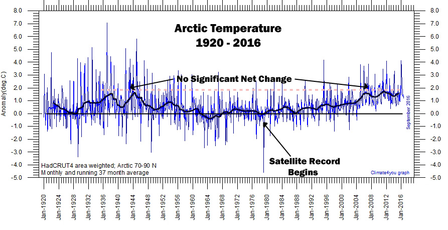
Apparently, Arctic sea ice volume was as low in the 1940s as it has been in the 2000s.
And the highest sea ice volume of the last 100 years was about 1979 – the year the Arctic sea ice record begins.🤔

Originally tweeted by Kenneth Richard (@Kenneth72712993) on January 24, 2021.
Here is the complete study published under a CC 4.0 License.
Brief communication: Arctic sea ice thickness internal variability and its changes under historical and anthropogenic forcing
The Cryosphere, 14, 3479–3486, 2020
https://doi.org/10.5194/tc-14-3479-2020
© Author(s) 2020. This work is distributed under
the Creative Commons Attribution 4.0 License.
Guillian Van Achter1, Leandro Ponsoni1, François Massonnet1, Thierry Fichefet1, and Vincent Legat2
- 1Georges Lemaitre Center for Earth and Climate Research, Earth and Life Institute, Université Catholique de Louvain, Louvain-la-Neuve, Belgium
- 2Institute of Mechanics, Materials and Civil Engineering, Applied Mechanics and Mathematics, Université Catholique de Louvain, Louvain-la-Neuve, Belgium
Correspondence: Guillian Van Achter ([email protected]) Received: 04 Dec 2019 – Discussion started: 10 Dec 2019 – Revised: 17 Jul 2020 – Accepted: 09 Sep 2020 – Published: 21 Oct 2020
Abstract
We use model simulations from the CESM1-CAM5-BGC-LE dataset to characterise the Arctic sea ice thickness internal variability both spatially and temporally. These properties, and their stationarity, are investigated in three different contexts: (1) constant pre-industrial, (2) historical and (3) projected conditions. Spatial modes of variability show highly stationary patterns regardless of the forcing and mean state. A temporal analysis reveals two peaks of significant variability, and despite a non-stationarity on short timescales, they remain more or less stable until the first half of the 21st century, where they start to change once summer ice-free events occur, after 2050.
How to cite. Van Achter, G., Ponsoni, L., Massonnet, F., Fichefet, T., and Legat, V.: Brief communication: Arctic sea ice thickness internal variability and its changes under historical and anthropogenic forcing, The Cryosphere, 14, 3479–3486, https://doi.org/10.5194/tc-14-3479-2020, 2020.1
Introduction
In the recent decades, Arctic sea ice has retreated and thinned significantly (Notz and Stroeve, 2016). The annual mean Arctic sea ice extent decreased by ∼2×10⁶ km2 between 1979 and 2016 (Onarheim et al., 2018). An analysis combining US Navy submarine ice draft measurements and satellite altimeter data showed that the annual mean sea ice thickness (SIT) over the Arctic Ocean at the end of the melt period decreased by 2 m between the pre-1990 submarine period (1958–1976) and the CryoSat-2 period (2011–2018) (Kwok, 2018). On long timescales (a few decades or more), retreating and thinning are projected to continue as greenhouse gas emissions are expected to rise. However, on shorter timescales (1–20 years), internal climate variability, defined as the variability of the climate system that occurs in the absence of external forcing and caused by the system’s chaotic nature, limits the predictability of climate (Deser et al., 2014) and represents a major source of uncertainty for climate predictions (Deser et al., 2012). In this context, greater knowledge of Arctic SIT internal variability and of its drivers is essential to document the true evolution of the Arctic atmosphere–ice–ocean system and to predict its future changes.
The mean spatial distribution of the Arctic SIT is relatively well documented (Stroeve et al., 2014). But there are some uncertainties around its interannual variability and its spatial modes of variability. Some studies (Lindsay and Zhang, 2006; Fuckar et al., 2016; Labe et al., 2018) already analysed the spatial distribution of Arctic sea ice variability by applying empirical orthogonal functions (EOFs) (K-means cluster analysis for Fuckar et al., 2016) to model-based historical SIT time series. Lindsay and Zhang (2006) reported a first mode nearly basinwide, while the second and third ones are orthogonal lateral modes accounting for 30 %, 18 % and 15 % of the variability, respectively. Fuckar et al. (2016) also found a nearly basinwide first mode, with an Atlantic–Pacific dipole as the second mode. Labe et al. (2018) depicted an Atlantic–Pacific dipole but as the first mode. The spatial structure and amount of explained variance of those modes are sensitive to whether and how the SIT time series is detrended. It is also model-dependent and influenced by the season and analysed period. The temporal sea ice volume (SIV) variability has been studied by Olonscheck and Notz (2017). These authors enlightened a remarkable similarity between the pre-industrial and historical internal variabilities of the annual Arctic SIV. They also noticed a decreased internal variability of winter and summer Arctic SIV for a future climate forced by the RCP8.5 scenario.
Apart from Olonscheck and Notz (2017), the studies cited above used data covering a few decades under historical forcing. In this work we use a long climate model control run under pre-industrial conditions from the CESM1-CAM5-BGC-LE dataset, which enables us to study only the internal variability of the Arctic SIT. We study the internal variability both temporally and spatially by applying a wavelet analysis and an EOF decomposition to the pan-Arctic SIV and gridded SIT anomaly time series, respectively. We also determine whether or not the SIV and SIT variability is stationary by analysing the model outputs under historical and future climate conditions with 30 ensemble members.
This paper is organised as follows. The model and its outputs are briefly described in Sect. 2. In Sect. 3, the spatial and temporal internal variability of Arctic sea ice is analysed, as well as its persistence through historical and future climate conditions. Then we explore the drivers of the main modes of internal variability. Conclusions are finally given in Sect. 4.
2 Data and methods
2.1 Sea ice thickness and volume datasets
We use the CESM1-CAM5-BGC-LE dataset (Kay et al., 2015). The Community Earth System Model Large Ensemble (CESM-LE) was designed to both disentangle model errors from internal climate variability and enable the assessment of recent past and future climate changes in the presence of internal climate variability. The CESM1(CAM5) is a CMIP5 participating model. It consists of coupled atmosphere, ocean, land and sea ice component models. It also includes a representation of the land carbon cycle, diagnostic biogeochemistry calculations for the ocean ecosystem and a model of the atmospheric carbon dioxide cycle (Moore et al., 2013; Lindsay et al., 2014). While it is not possible to validate the data in terms of SIT and SIV variabilities due to the lack of continuous observational data, the model was well validated in terms of mean state of the ice thickness and extent, as well as regarding the recent trends in the latter. Jahn et al. (2016) showed good agreement between observations and CESM1(CAM5) simulations for mean Arctic sea ice thickness and extent in the early 21st century. Barnhart et al. (2016) demonstrated that CESM1(CAM5) captures the trend of declining Arctic sea ice extent over the period of satellite observations. Based on these validation studies, we consider that the CESM1-CAM5-BGC-LE time series is a fair proxy to study the variabilities of the Arctic SIT and SIV under different forcing conditions.
In this paper, we use the monthly averaged Arctic SIT and SIV provided over the three periods (pre-industrial, historical and future). The pre-industrial period is represented by a single 1700-year control simulation with constant pre-industrial forcing. The ocean model was initialised from a state of rest (Danabasoglu et al., 2012), while the atmosphere, land and sea ice models were initialised using previous CESM1(CAM5) simulations. This experimental design allows the assessment of internal climate variability in the absence of climate change. In practical terms, we will use the last 200 years of this simulation. The historical period has one ensemble member covering the 1850–2005 period and 30 ensemble members over 1920–2005. Also with 30 ensemble members, the future climate period (2006–2100) follows the Representative Concentration Pathway (RCP) 8.5 scenario, corresponding to a total radiative forcing of 8.5 W m−2 in 2100 relative to pre-industrial conditions (Meinshausen et al., 2011). The Canadian Archipelago region was removed from the dataset since SIT reaches unrealistic values in this area.
For the variability analysis, the trend and seasonal cycle are removed from the time series (pan-Arctic SIV and gridded SIT) so that we focus on the interannual variability. Since the spatial variability analysis uses 30 ensemble members, the SIT anomaly fields are computed by removing the ensemble mean to each member. When only one ensemble member is used, as for the temporal analysis, the anomaly is calculated by excluding the individual trend (provided by a second-order polynomial fit) of each month.
2.2 Variability analysis
To characterise the internal variability of the Arctic sea ice, we aim at inspecting how the SIV variability evolves in time and how SIT variability is characterised in space. For addressing the temporal variability, we make use of wavelet analysis, with Morlet as wavelet mother, following the methodology proposed by Torrence and Compo (1998). The wavelet analysis has the advantage of taking into account possible non-stationarity of the time series. In this paper, we show the results for one of the historical (1850–2005) members and one of the future (2006–2100) members, although we tested the robustness of the results over the 30 ensemble members as discussed later (Sect. 3.1 and 3.2).
The spatial variability is analysed by computing the EOFs on the SIT anomaly time series. This decomposition reduces the large number of variables of the original data to a few variables, but without compromising much of the explained variance. Each EOF represents a mode of SIT variability that provides a simplified representation of the state of the SIT at that time along that EOF. In other words, the EOFs themselves are fixed in time but their weighting coefficients are time-varying; the associated time series (one for each mode) indicate in which state the SIT is at any time (Hannachi, 2004). The analysis is made on the gridded SIT anomaly time series for the three periods. For the historical and future periods, the EOFs are computed over 30 ensemble members, all appended together over time (as done by Labe et al., 2018).
By applying those analyses separately over the three periods, we aim to document the internal variability in the absence of any external forcing during the pre-industrial period. By comparing the pre-industrial results with those for the historical and future periods, we estimate the evolution of the SIT and SIV internal variability under anthropogenic forcing.
3 Results
3.1 Temporal variability
The results from the wavelet analysis are presented in Fig. 1a–c, in which the wavelet power spectrum is shown as a function of time (bottom left of each subfigure). On the wavelet power spectrum, the crosshatched area denotes the “cone of influence”, in which edge effects become important, and the red lines denote the 95 % significance levels above a red noise background spectrum. The global wavelet spectrum is also shown (bottom right), which is a time-integrated power of the wavelet power spectrum. The significance level of the time-integrated wavelet spectrum is indicated by the dashed curve. It refers to the power of the red noise level at the 95 % confidence level that increases with decreasing frequency.
The temporal variability of the Arctic SIV anomaly over the pre-industrial period is depicted in Fig. 1a. The time-integrated power spectrum (bottom right) shows two peaks of significant variability. The first peak corresponds to a period centred on 8 years but spanning from 5 to 10 years. The second one corresponds to a period of 16 years spanning from 10 to 20 years. In the wavelet power spectrum, the red lines enclose regions in which the variability is significant. The two main peaks are present throughout the time span, but not always concomitantly. Depending on the time, both the 8- and 16-year periods are significant, with one of them appearing stronger in the power spectrum (Fig. 1a, bottom left panel). For instance, the 8-year peak is dominant during the 1780–1810 period, the 16-year peak during the 1750–1780 period and both peaks during the 1830–1850 period.
Over the historical period, the Arctic SIV temporal variability shows a first peak centred on 5 years and two others centred on 10 and 16 years, all with 95 % confidence (Fig. 1b). The wavelet power spectrum shows that the 16-year period is significant throughout the entire time span, while the 8-year period loses significance around certain periods of time (e.g. around 1925). The future climate SIV wavelet analysis in Fig. 1c presents a clear loss of variability after the year 2050. This loss of variability is visible in the SIV time series and is confirmed by both the wavelet power spectrum and the time-integrated power spectrum. The 2050 sudden loss of variability coincides with the ice-free summer events occurring at that time. Apart from that loss of variability, the wavelet power spectrum exhibits one band of 5-year variability during the 2015–2025 period and another band of 10-year variability during the 2025–2050 period, both bands with 95 % confidence. In Fig. 1c, the peaks are not significant on the time-integrated power spectrum because the respective variability is significant only over the first 50 years as is shown in the wavelet power spectrum (areas in red).
The main characteristics of the temporal variability of the Arctic SIV under pre-industrial conditions seem to persist under anthropogenic forcing. The two major temporal peaks of variability centred on 8 and 16 years, found in the pre-industrial run, are also present during the historical period. For the first half of the 21st century, the future projections are also dominated by the two main peaks but centred at 5 and 10 years in the integrated spectrum, and with relatively weaker power compared to the pre-industrial and historical runs. Furthermore, the SIV variability seems to be non-stationary since the power is not always above the 95 % significance level.
The wavelet analyses applied to the other 30 ensemble members of the historical and future simulations bring robustness to our results since, overall, each member shows a similar pattern of temporal variability. To promote such a multi-member comparison among the different spectra, we have first normalised all spectra (and the significance curve) by their respective maximum value so that the power ranges from 0 to 1. This step is required to make the spectrum from each member have the same weight in the averaging. As shown in Fig. 1d (blue line), the averaged spectrum is smoothed out across the time domain because the peaks from different spectra are not co-located exactly at the same periods. Nevertheless, it still shows that the variability is significant over the background red noise (see dashed red line). To complement this analysis, we have counted the number of local peaks for each period and from all 30 spectra. As shown by the black line in Fig. 1d, there is a concentration of peaks around the 8-year and 22-year periods. This spread compared to the reference historical run is somehow expected since the internal variability between the different members is not expected to be identical and even tends to increase with time (Blanchard-Wrigglesworth et al., 2011). For members covering the 21st century, the results are close to the one-member analysis discussed above.
3.2 Spatial variability
The spatial variability of the Arctic SIT anomaly is depicted by the major modes of variability in Fig. 2. Since the SIV exhibits a strong loss of variability around the year 2050, the future period for this spatial variability analysis spans from 2006 to 2050. For each period, the modes are sorted by percentage of variability explained. The first mode, which explains most of the variability, represents 22 %, 20 % and 20 % of the variability for pre-industrial, historical and future climate conditions, respectively. All periods show the same pattern of SIT spatial variability for the first mode. It corresponds to a dipole between the Fram Strait area and the East Siberian Sea (Fig. 2a, b, c). For both the pre-industrial and historical periods, the second mode of variability is a pole centred in the East Siberian Sea, but also spreading into the Arctic Basin (Fig. 2d, e). It accounts for 14 % and 11 % of the variability, respectively. The third mode of variability for the pre-industrial period corresponds to a dipole between the Laptev and Kara seas, on the one hand, and the east coast of Greenland, the Chukchi Sea and Beaufort Sea, on the other hand.

Figure 2 Modes of Arctic SIT spatial variability. From the left to the right, each row shows the first three EOFs of Arctic SIT over the pre-industrial (200 years preceding the historical integration) (a, d, g), historical (1920–2005) (b, e, h) and future (2006–2050) (c, f, i) periods, respectively. EOFs for the historical and future periods are performed over 30 ensemble members.
The first mode of SIT is stable over time and stays the dominant mode of spatial variability in all three periods. There are some disparities in percentage explained and in magnitude, which could be explained by the different lengths of the periods. As the first mode, the second mode of SIT spatial variability is persistent in the historical period. For the future climate period, the second mode of SIT variability is no longer persistent. It presents a dipole of variability as the first mode, but the Pacific part of the dipole is larger and no longer located in the East Siberian Sea. The third modes of the three periods (Fig. 2g, h, i) exhibit all different patterns of variability and they are not considered in further analysis.
After 2050, the SIT spatial variability is impacted by the sudden decrease in SIT. EOFs computed over the 2050–2100 period (not shown) exhibit the same pattern of the dipole as the first mode for the 2005–2050 period, but the area of high variability is not the same. The Atlantic part of the dipole is shifted toward the north coast of Greenland, and the Pacific part of the dipole is also reduced near the coast.

Figure 3 Arctic sea ice mean circulation during low (a) and high (b) indices of the first mode of SIT variability during the pre-industrial period. Arctic mean surface air temperature anomaly during low (c) and high (d) indices of the second mode of SIT variability.
3.3 Drivers of the major modes of SIT internal variability
By computing the temporal oscillation between phases of a certain mode of variability, we are able to characterise this mode by low and high indices. In order to find the physical drivers of the SIT modes of variability, we investigate the differences in dynamic and thermodynamic features (sea ice velocity, atmospheric surface temperature) between both phases of the modes. Figure 3a, b show the mean Arctic sea ice circulation over the pre-industrial period by compositing the low (a) and high (b) indices for the first mode of SIT variability. The sea ice drift anomaly associated with the positive and negative phases of the first SIT mode shares similar features with the Arctic Oscillation: a cyclonic anomaly in the Beaufort Gyre, impacting the Transpolar Drift Stream, the Laptev Sea Gyre and the East Siberian circulation, as described by Rigor et al. (2002).
Furthermore, applying wavelet analysis to the associated time series of the first spatial mode of variability indicates that the main periodicity of this mode is centred on 8 years and spans from 5 to 10 years (not shown). This result is suggestive of a link between the first mode of temporal variability of the wavelet analysis and the first mode of spatial variability, and so to the Arctic Oscillation.
We also used the associated time series of the second mode of SIT spatial variability to characterise it by low and high indices. The same analysis over the sea ice velocity is performed for the second mode. For both indices, the sea ice velocity fields are similar. We concluded that the second mode is not dynamically driven. Following Olonscheck et al. (2019) results, which demonstrate that the internal variability of Arctic sea ice area and concentration are primarily caused by atmospheric temperature fluctuations, we investigated the differences in mean surface air temperature anomaly over the pre-industrial period between the low and high indices for both the first and second modes of SIT variability. Two widely different states of surface air temperature are found between indices for both modes (the surface air temperature anomaly for the second mode is depicted in Fig. 3c, d). It appears that the SIT variability and the surface air temperature are associated with each other.
4 Conclusions
In this work, we have analysed the internal variability of the Arctic SIT both spatially and temporally with the CESM1-CAM5-BGC-LE dataset. We conducted wavelet analysis of the pan-Arctic SIV anomaly and EOF decomposition of the gridded SIT anomaly, both over a 200-year control run conducted under pre-industrial conditions. Then, to assess the persistence of the SIT anomaly internal variability under anthropogenic forcing, we performed the same analyses with 30 ensemble members over the historical and future periods.
The temporal analysis of the SIV anomaly internal variability shows two peaks of significant variability. One centred on 8 years, spanning from 5 to 10 years, and another one centred on 16 years, spanning from 10 to 20 years. These two peaks of temporal variability are present in both the pre-industrial and historical periods, as well as in the first half of the 21st century. After that, a sudden loss of variability due to ice-free summer events is found. Furthermore, despite a dominant periodicity over the three periods, the SIV anomaly has been observed to be non-stationary. Indeed, the dominant periodicity of the SIV variability can be centred on either 8 or 16 years, depending on the timescale and period. Wavelet analyses over the 30 ensemble members for the post-industrial period have shown the same behaviour of temporal variability within members, except that the peaks are not always centred in 8 and 16 years but somewhere between 5–10 and 15–26 years, depending on the member.
The spatial analysis of the SIT anomaly internal variability has been applied to the 30 ensemble members and reveals two important modes of variability. The first one is a mode with opposite signs centred in the East Siberian Sea and in the Fram Strait area, accounting for 22 % of the variability in the pre-industrial period. This first mode is a dynamical one, related to the Arctic Oscillation, and persists over all pre-industrial, historical and future periods. Furthermore, this first mode of spatial variability has a temporal variability of 8 years (spanning from 5 to 10 years), corresponding to the first peak of variability found in the temporal analysis. The second mode exhibits a large pole of variation centred on the East Siberian Sea going through the Arctic Basin. It represents 14 % of the variability in the pre-industrial period.
The loss of sea ice in summer starting in 2050 and the strong decrease in SIV in winter during the second half of the 21st century (from 15 to 10×103 km3) strongly modifies the variability of the ice both spatially and temporally. The main modes of spatial variability lose their significance or just disappear after 2050, and the temporal analysis shows a total disappearance of the variability at that time.
This analysis of the Arctic SIT and SIV variability bears some limits. Indeed, our results for the temporal and spatial patterns of variability are based on only one model, and despite the use of 30 ensemble members and a reasonable validation against observations, the model is not perfect. Furthermore, the spatial modes of SIT variability are robust for all the 30 ensemble members, but the temporal analysis shows some dissimilarities between members. Other studies with other model outputs are therefore needed to confirm our conclusion.
Finally, in the context of recent climate changes, predicting sea ice has never been so important. However, to validate and improve our predictions, observational data are crucial. In this sense, our variability analysis of internal SIV and SIT variability might help the development of an optimal sampling strategy, taking into account the selection of well-placed sampling locations for monitoring the SIT and, therefore, the pan-Arctic SIV that are not as well documented as the sea ice extent and area (Ponsoni et al., 2020).
Code availability.
The wavelet analysis is performed with the Waipy module on Python (https://github.com/mabelcalim/waipy, last access: 1 March 2020).
Data availability.
Data can be downloaded from the following source:
https://www.earthsystemgrid.org/dataset/ucar.cgd.ccsm4.CESM_CAM5_BGC_LE.ice.proc.monthly_ave.html
(last access: 1 March 2020). The 30 ensemble members used in this study are the first 30 members (001-030).
Author contributions. GVA, LP, FM, TF and VL designed the science plan. GVA conducted the data processing, produced the figures, analysed the results and wrote the manuscript based on the insights from all co-authors.
Competing interests. The authors declare that they have no conflict of interest.
Acknowledgements. François Massonnet and Leandro Ponsoni are a F.R.S.-FNRS research associate and a post-doctoral researcher, respectively. Guillian Van Achter is funded by the PARAMOUR project which is supported by the Excellence Of Science programme (EOS), also founded by FNRS. We thank the two referees for their very helpful comments on an earlier version of this paper.Financial support.
The work presented in this paper has received funding from the European Commission, H2020 Research Infrastructures (APPLICATE project – Advanced prediction in Polar regions and beyond, grant no. 727862 and PRIMAVERA project – PRocess-based climatesIMulation: AdVances in high-resolution modelling and Europeanclimate Risk Assessment, grant no. 641727).
Review statement. This paper was edited by Michel Tsamados and reviewed by two anonymous referees.
References
Barnhart, K. R., Miller, C. M., Overeem, I., and Kay, E.: Mapping the future expansion of Arctic open water, Nat. Clim. Change, 6, 280–285, https://doi.org/10.1038/NCLIMATE2848, 2016.
Blanchard-Wrigglesworth, E., Bitz, C. M., and Holland, M. M.: Influence of Initial Conditions and Climate Forcing on Predicting Arctic Sea Ice, Geophys. Res. Lett., 38, L18503, https://doi.org/10.1029/2011GL048807, 2011.
Danabasoglu, G., Bates, S. C., Briegleb, B. P., Jayne, S. R., Jochum, M., Large, W. G., Peacock, S., and Yeager, S. G.: The CCSM4 ocean component, J. Climate, 25, 1361–1389, https://doi.org/10.1175/JCLI-D-11-00091.1, 2012.
Deser, C., Philips, A. S., Alexander, M. A., and Smoliak, B. V.: Projecting North American Climate over the Next 50 Years: Uncertainty due to Internal Variability, J. Climate, 27, 2271–2296, https://doi.org/10.1175/JCLI-D-13-00451.1, 2014.
Deser, C., Philips, A., Bourdette, V., and Teng, H.: Uncertainty in climate change projections: the role of internal variability, Clim. Dynam., 38, 527–546, https://doi.org/10.1007/s00382-010-0977-x, 2012.
Fučkar, N. S., Guemas, V., Johnson, N. C., Massonnet, F., and Doblas-Reyes, F.: Clusters of Interannual Sea Ice Variability in the Northern Hemisphere, Clim. Dynam., 47, 1527–1543, https://doi.org/10.1007/s00382-015-2917-2, 2016.
Hannachi, A.: A Primer for EOF Analysis of Climate Data, Department of Meteorology, University of Reading Reading, 2004.
Jahn, A., Kay, J. E., Holland, M. M., and Hall, D. M.: How predictable is the timing of a summer ice-free Arctic?, Geophys. Res. Lett., 43, 9113–9120, https://doi.org/10.1002/2016GL070067, 2016.
Kay, J. E., Deser, C., Phillips, A., Mai, A., Hannay, C., Strand, G., Arblaster, J. M., Bates, S. C., Danabasasoglu, D., Edwards, J., Holland, M., Kushner, P., Lamarque, J.-F., Lawrence, D. , Lindsay, K., Midd Leton, A., Munoz, E., Neale, E., Oleson, K., Polvani, L., and Vertenstein, M.: The Community Earth System Model (CESM) Large Ensemble Project, A Community Resource for Studying Climate Change in the Presence of Internal Climate Variability, B. Am. Meteorol. Soc., 96, 1333–1349, https://doi.org/10.1175/BAMS-D-13-00255.1, 2015.
Kwok, R.: Arctic sea ice thickness, volume, and multiyear ice coverage: losses and coupled variability (1958–2018), Environ. Res. Lett., 13, 10, https://doi.org/10.1088/1748-9326/aae3ec, 2018.
Labe, Z., Magnusdottir, G., and Stern, H.: Variability of Arctic Sea Ice Thickness Using PIOMAS and the CESM Large Ensemble, J. Climate, 31, 3233–3247, https://doi.org/10.1175/JCLI-D-17-0436.1, 2018.
Lindsay, K., Bonan, G. B., Doney, S. C., Hoffman, F. M., Lawrence, D. M., Long, M. C., Mahowald, N. M., Moore, J. K., Randerson, J. T., and Thornton, P. E.: Preindustrial-control and twentieth-century carbon cycle experiments with the Earth system model CESM1(BGC), J. Climate, 27, 8981–9005, doi.org/10.1175/JCLI-D-12-00565.1, 2014.
Lindsay, R. W. and Zhang, J.: Arctic Ocean Ice Thickness: Modes of variability and the Best Locations from Which to Monitor Them, J. Phys. Oceanogr., 36, 496–506, https://doi.org/10.1175/JPO2861.1, 2006.
Meinshausen, M., Calvin, S. J., Daniel, J. S., Kainuma, M. L. T., Lamarque, J.-F., Matsumoto, K., and Montzka, S. A.: The RCP greenhouse gas concentrations and their extensions from 1765 to 2300, Climatic Change, 109, 213–241, https://doi.org/10.1007/s10584-011-0156-z, 2011.
Moore, C. P., Lindsay, K., Doney, S. C., Long, S. C., and Misumi, K.: Marine ecosystem dynamics and biogeochemical cycling in the Community Earth System Model[CESM1(BGC)]: Comparison of the 1990s with the 2090s under the RCP4.5 and RCP8.5 scenarios, J. Climate, 26, 9291–9312, https://doi.org/10.1029/2011JD017187, 2013.
Notz, D. and Stroeve, J.: Observed Arctic sea-ice loss directly follows anthropogenic CO2 emission, Science, 354, 747–750, https://doi.org/10.1126/science.aag2345, 2016.
Olonscheck, D. and Notz, D.: Consistently estimating internal climate variability from climate-model simulations, J. Climate, 30, 9555–9573, https://doi.org/10.1175/JCLI-D-16-0428.1, 2017.
Olonscheck, D., Mauritsen, T., and Notz, D.: Arctic Sea-Ice Variability Is Primarily Driven by Atmospheric Temperature Fluctuations, Nat. Geosci., 12, 430–434, https://doi.org/10.1038/s41561-019-0363-1, 2019.
Onarheim, I. H., Eldevik, T., Smedsrud, L. H., and Stroeve, J. C.: Seasonal and Regional Manifestation of Arctic Sea Ice Loss, J. Climate, 31, 4917–4932, https://doi.org/10.1175/JCLI-D-17-0427.1, 2018.
Ponsoni, L., Massonnet, F., Docquier, D., Van Achter, G., and Fichefet, T.: Statistical predictability of the Arctic sea ice volume anomaly: identifying predictors and optimal sampling locations, The Cryosphere, 14, 2409–2428, https://doi.org/10.5194/tc-14-2409-2020, 2020.
Rigor, I. G., Wallace, J. M., and Colony, R. L.: Response of Sea Ice to the Arctic Oscillation, J. Climate, 15, 2648, https://doi.org/10.1175/1520-0442(2002)015<2648:ROSITT>2.0.CO;2, 2002.
Stroeve, J., Barrett, A., Serreze, M., and Schweiger, A.: Using records from submarine, aircraft and satellites to evaluate climate model simulations of Arctic sea ice thickness, The Cryosphere, 8, 1839–1854, https://doi.org/10.5194/tc-8-1839-2014, 2014.
#
Related links:
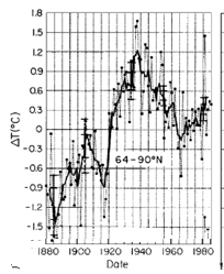
Arctic Temperatures…
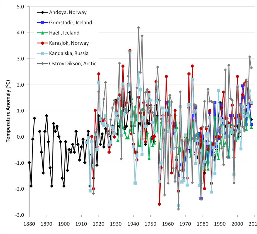
With live evidence of rapid decline before 1940
then rapid growth in the 1970s
Also with DOE data…
And Hanson’s early “before-the-con” data
And HAD4 Arctic sea surface temperatures
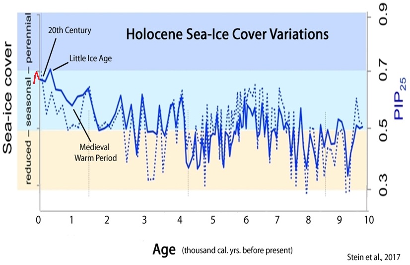
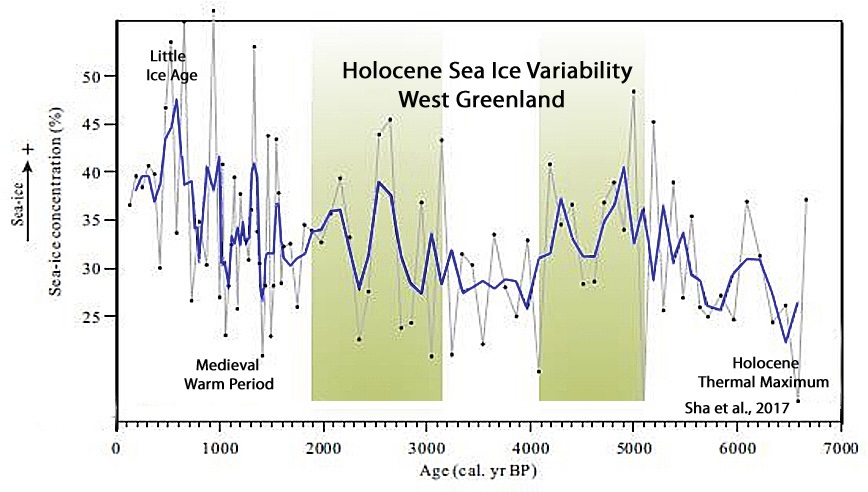
biological proxy data from all over the Arctic shows that for most of the last 10,000 years,
…. sea ice extent has been MUCH LOWER THAN CURRENT LEVELS
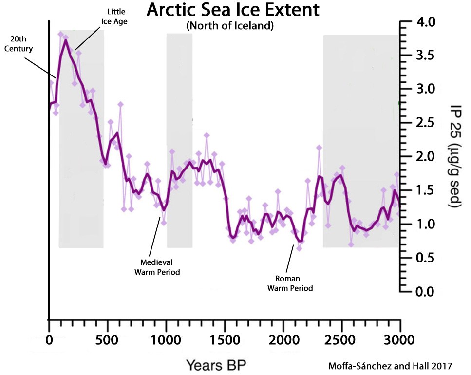
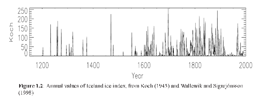
Icelandic Sea ice charts show the 1970s extents being up with the EXTREME high levels of the LIA